FlexCel API Developer Guide

Introduction

The FlexCel API (Application Programmer Interface) is what you use to read or write Excel files in a low-level way. By “low-level” we mean that this API is designed to work really “close to the metal” and there aren’t many layers between you and the xls/xlsx file being created. For example, FlexCel API doesn’t know about datasets, because datasets are a higher level concept. If you want to dump a dataset into an Excel file using the API, you need to loop in all records and enter the contents into the cells.

In addition to the FlexCel API we provide a higher level abstraction, TFlexCelReport, that knows about datasets and in general works at a more functional level; a declarative approach instead of an imperative approach. What is best for you depends on your needs.

Basic Concepts

Before starting writing code, there are some basic concepts you should be familiar with. Mastering them will make things much easier down the road.

Arrays and Cells

To maintain our syntax compatible with Excel OLE automation, most FlexCel indexes/arrays are 1-based.

That is, cell A1 is (1,1) and not (0,0). To set the first sheet as ActiveSheet, you would write ActiveSheet := 1 and not ActiveSheet := 0.

So, in C++ loops should read: for (int i = 1; i <= Count; i++), and in Delphi they should be like for i := 1 to Count.

The two exceptions to this rule are XF and Font indexes, which are 0 based because they are so in Excel.

Cell Formats

All formats (colors, fonts, borders, etc.) on an Excel workbook are stored into a list, and referred by number. This number is known as the XF (eXtended Format) index. A simple example follows:

Here Cell B3 has XF = 0 and the XF definition for the background color is green. Row 6 has XF = 2, so all the empty cells on row 6 are orange. Column C has XF = 1, so all the empty cells on column C that do not have a Row Format are blue.

The priority goes, from higher to lower: Cell format->Row format->Column format. This means that if column A has a column format red and Row 1 has row format green, the cell A1 will be green. If you apply a cell format to cell A1, it will be used instead of either row or column formats as it has the highest priority.

Note

Sometimes when you work in Excel, it might look like Excel is handling priority differently. For example if you format a row green and after that a column red, you will see that the intersection between the column and row is red.

What is happening under the hood is that when you format the column red, Excel applies a column format red to the column, and after that a cell format red to the cell in the intersection. This way it can look like the column format is taking priority over the row, but it is actually the cell format applied to the cell at the intersection which has the priority.

Most formatting methods at FlexCel return an XF index, and then you have to look at the XF list (using the TExcelFile.GetFormat method) to get a class encapsulating the real format. There is a helper method: TExcelFile.GetCellVisibleFormatDef that obtain the XF index and return the format class in one step.

To create new formats, you have to use the TExcelFile.AddFormat method. Once you get the Id of the new XF, you can use it as you wish.

Note

You don't have to worry also on inserting a format 2 times: If it already exists AddFormat will return the existing id and not add a new XF entry.

Cell and Style Formats

XF formats can be of two types, “Cell” or “Style”. Cell formats are applied directly to a cell and can have a “ParentStyle” which must be a style format. Style formats cannot have ParentStyle and cannot be applied to cells, but they can be used as the base for defining different Cell formats. You can know if a TFlxFormat contains a “Style” or “Cell” format by looking at its “IsStyle” property. Also, a cell style can link only parts of its format to its parent style, for example have the font linked so when you change the font in the style it changes the font in the cell, but not the cell borders. In order to set which properties are linked to the main style, you need to change the “LinkedStyle” property in TFlxFormat.

You can create new Style formats with TExcelFile.SetStyle, and new Cell formats with TExcelFile.AddFormat. Once you create a new style and give it a name, you can get its definition as a TFlxFormat, change its TFlxFormat.IsStyle property to true, define which properties you want to link with the TFlxFormat.LinkedStyle property, and add that format using AddFormat to get the cell format. Once you have the cell style, you can just apply it to a cell.

Note

The TLinkedStyle record has a member, TLinkedStyle.AutomaticChoose, which if left to true (the default) will compare your new format with the style and only link those properties that are the same.

For example, let’s imagine you create a style “MyHyperlink”, with font blue and underlined. Then you create a Cell format that uses “MyHyperLink” as parent style, but also has a red background, and apply it to cell A1. If you leave AutomaticChoose true, FlexCel will detect that the cell format is equal in everything to its parent style except in the background, so it will not link the background of the cell to the style. If you later change the background of MyHyperlink, cell A1 will continue to be red.

This allows for having “partial styles” as in the example above: a “hyperlink” style defines that text should be blue and underlined, but it doesn’t care about the cell background. If you want to manually set which properties you want to have linked instead of FlexCel calculating that for you, you need to set TLinkedStyle.AutomaticChoose to false and set the “Linked….” Properties in TLinkedStyle to the values you want.

Font Indexes

The same way we have an XF list where we store the formats for global use, there is a Font list where fonts are stored to be used by XFs. You normally don't need to worry about the FONT list because inserting on this list is automatically handled for you when you define an XF format. But, if you want to, you can for example change Font number 7 to be 15 points, and all XFs referencing Font 7 will automatically change to 15 points.

Colors

While colors in Excel up to 2003 were indexes to a palette of 56 colors, Excel 2007 introduces true colors, and FlexCel implements it too since version 5.0. One thing that is nice about the new colors is that they can be retrofitted in the xls file format, so while you won’t be able to see true color in Excel 2003 (Excel 2003 just doesn't know about them), the data is there in the xls file anyway. So if you open the xls file with FlexCel 5 or later Excel 2007 and later you will see the true colors, even if the xls file format originally didn't know about them.

There are four kinds of colors that you can use in Excel:

• RGB: This is just a standard color specified by its Red, Green and Blue values.

• Theme: There are 12 theme colors, and each of them can have a different tint (brightness) applied. Theme colors are the default in newer Excel versions and you are likely using them even if not aware.

  Given the importance of theme colors in newer Excel, and that they aren't trivial to describe, we will cover them in a separate section below.

• Indexed Colors. This is kept for background compatibility with Excel 2003, but we strongly recommend you forget about them.

• Automatic Color. An automatic color changes depending on whether the color is used as a background or as a foreground. For foreground colors (like a font color) the Automatic color is black. For background colors (like a cell back color) the automatic color is white

You can access any of these variants with the record TExcelColor.

TExcelColor also automatically converts from a system TColor, so you can just specify something like:

MyObject.Color = clBlue;

If you want to use a theme color, you will have to use:

MyObject.Color = TExcelColor.FromTheme(…);

The “NearestColorIndex” used in older version of FlexCel has been deprecated and you shouldn’t use it.

Theme colors

Theme colors are an interesting topic well worth its own section in this manual. Excel uses theme colors by default, which means that most spreadsheets you see around are using them, even if the people who created the files didn't know what a "theme" color was.

The first thing to notice is that Excel has 12 theme colors, which FlexCel maps inside the TThemeColor enumeration. Each one of those 12 colors can be made lighter or darker by changing its TExcelColor.Tint leading to millions of possible colors derived from those basic 12 colors.

When you open a color dialog in Excel, the colors that are shown in the main square are different variations of the 12 theme colors:

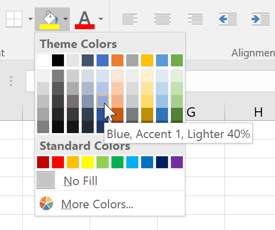
Each one of the 12 theme colors takes one column in the grid, and in the rows of the grid you can see variations of those colors with different tints.

Note

We kind of lied here: If you tried to count the columns in the image, you would see that there are 10 columns instead of 12. This is because even when Excel has 12 defined theme colors, only 10 of them are visible. The other 2 are the color for a hyperlink and a visited hyperlink, and they don't show in the Excel UI as usable colors.

The selected color you see in the image above is a color of the theme Accent1 (all colors in column 4 are of theme Accent1). It also has applied a tint which makes it 40% lighter than the standard Accent1 color, as shown in the Excel tooltip.

Themes are a nice way to specify colors, since you can change the theme later, and all colors will change to match. This means that you can go to the theme selector in the Excel ribbon (in the Page Layout tab) and change what Accent1 (and all the other theme colors) mean:

If you select for example the "Ion Boardroom" theme as shown in the image, you will see the color palette changes to:

Note how the color Accent1 is now Plum instead of Blue. When you change the theme of your spreadsheet, all cells which had Accent1 theme colors will change from blue to plum, while cells which had a Blue RGB color set will continue to be blue.

When setting colors in a file you are creating, it is a nice thing to use theme colors instead of RGB colors, so your users will be able to change the theme. FlexCel has full support of theme colors, and you can easily find out how to use them in your code with APIMate.

You can find more information about Excel 2007 colors at

http://tmssoftware.com/site/blog.asp?post=135

Date Cells

As you might already know, there is no DATE datatype in Excel.

Dates are saved as a double floating number where the integer part is the number of days that have passed from 1/1/1900, and the fractional part is the corresponding fraction of the day. For example, the number 2.75 stands for "02/01/1900 06:00:00 p.m." You can see this easily at Excel by entering a number on a cell and then changing the cell format to a date, or changing the cell format of a date back to a number.

The good news is that you can set a cell value to a DateTimeValue, and FlexCel will automatically convert the value to a double, keeping in count “1904” date settings (see below). That is, if you enter

XlsFile.SetCellValue(1, 1, Now), and the cell (1,1) has date format, you will write the actual value of "now" to the sheet.

The bad news is that you have no way to know if a cell has a number or a date just by looking at its value. If you enter a date value into a cell and then read it back, you will get a double. So you have to look at the format of the cell. There is a helper function, FormatValue that can return if the cell has a date or not by looking at the format.

Important

TExcelFile.GetCellValue will return a TCellValue record and TCellValue has a ValueType which can be of type TCellValueType.DateTime.

So it might be tempting to write code like this:

var
  CellValue: TCellValue;
...
  CellValue := xls.GetCellValue(row, col);

  //This is WRONG. CellValue.IsDateTime is always false
  //when reading values from a sheet.
  //The dates you see in the sheet are just numbers with
  //a date format, so their ValueType is Number.
  if CellValue.IsDateTime then
  begin
    LogMessage(('Cell ' + TCellAddress.Create(row, col).CellRef) + ' contains a Date and Time');
  end;

Sadly this code won't work. In Excel dates are stored as numbers, so the ValueType FlexCel will return for a cell with a date will be Number, not DateTime. TCellValueType.DateTime exists only for setting values into FlexCel (so you can write xls.SetCellValue(row, col, Now) and FlexCel can manage to correctly enter the datetime with the 1904 settings of the file).

But TCellValueType.DateTime won't help when reading files and trying to figure out if a cell contains a date. The only way to find out that is by looking at the format of the cell.

This would be the correct way to find out if a cell contains a date:

var
  fmt: TFlxFormat;
...
  fmt := xls.GetCellVisibleFormatDef(row, col);
  if TFlxNumberFormat.HasDateOrTime(fmt.Format) then
  begin
    LogMessage(('Cell ' + TCellAddress.Create(row, col).CellRef) + ' contains a Date and Time');
  end;

  if TFlxNumberFormat.HasDate(fmt.Format) then
  begin
    LogMessage(('Cell ' + TCellAddress.Create(row, col).CellRef) + ' contains a Date');
  end;

  if TFlxNumberFormat.HasTime(fmt.Format) then
  begin
    LogMessage(('Cell ' + TCellAddress.Create(row, col).CellRef) + ' contains a Time');
  end;

Note how the actual value of the cell doesn't matter, only the format of the cell.

Note

Excel also has a “1904” date mode, where dates begin at 1904 and not 1900. This mode was used on Excel for mac before OSX: today both OSX and Windows use a 1900 date system. But you can change this option in Excel for OSX or Windows today too, so you might come across some file using the 1904 date system. FlexCel completely supports 1900 and 1904 dates, but you need to be careful when converting dates to numbers and back.

You can read more information here: https://support.microsoft.com/en-us/help/214330/differences-between-the-1900-and-the-1904-date-system-in-excel

Note

There is a bug in how Excel handles the 1900 year. It considers it to be a leap year but 1900 was a normal year and February 29 1900 never happened. This means that the serial number used to represent the date gets one day out of sync with the serial number used by Delphi. The serial number 0 will show in Excel as "January 0, 1900" (even if there was never a January 0 either)

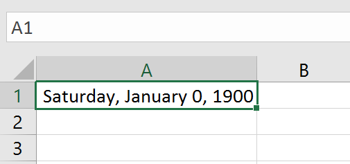
While in Delphi it will show as December 30, 1899

Note that even if Excel cared to display correctly the 0 as December 31, 1899 instead of January 0, 1900 it would still be off by a day with the dates as used in Delphi, which displays December 30.

FlexCel will try to do the best to replicate the Excel bug so you get the same values as Excel (ironically, Excel has the bug only because it was replicating a bug in Lotus 1-2-3). This means that for example TFlxDateTime.FromOADate(0, false) will return a TDateTime of January 31, 1899 which is the closest we can get to the value Excel shows. (we can't return a TDateTime with a value of January 0, that is not possible). But whatever we do, the reality is that dates in Excel before March 1, 1900 are wrong. Avoid using them.

You can read more information on this bug here. https://support.microsoft.com/en-us/help/214326/excel-incorrectly-assumes-that-the-year-1900-is-a-leap-year

Copying and pasting native Excel data

TExcelFile has a group of methods that allow you to copy/paste from/to FlexCel to/from Excel in native Excel format (Biff8). You can copy data to the clipboard in Biff8, Tabbed Text, and HTML formats. You can paste from the clipboard in BIFF8 and Tabbed-Text format.

Normally copying in Biff8 is good for pasting the data in Excel, Html is good if you later want to paste in Word or PowerPoint, and text works for pasting into applications that don’t understand Biff8 or HTML.

Copying and pasting in native BIFF8 format is a great advance over copying/pasting on plain text only. It allows you to keep cell formats/colors/rounding decimals/merged cells/etc. But it has its limitations too:

• It can't copy/paste images

• It can't copy/paste strings longer than 255 characters

• It can't copy the data on multiple sheets.

We would like to say that these limitations are not FlexCel's fault. The BIFF8 specification is correctly implemented; those are limitations on Excel's part.

Of course, Excel can copy and paste everything without problems, but this is because Excel doesn't use the clipboard to do the operation. If you close all instances of Excel, open a Worksheet, copy some cells to the clipboard, close Excel and open it again you will run into the same limitations. Copy/paste limitations on Excel don't show when it is kept in memory.

Reading and Writing Files

The native FlexCel engine is encapsulated on the class TXlsFile.

This class stores an Excel file in memory, and has methods allowing loading a new file into it, modifying it, or saving its contents to a file or a stream.

Note

TExcelFile is the abstract class that provides the interface that TXlsFile implements. In this documentation, we use TExcelFile and TXlsFile interchangeably, because both implement the same methods and properties. The first is an abstract class which specifies the functionality, and the second is the actual code.

Important

Keep in mind that a TXlsFile object stores a full spreadsheet in memory. Do not leave global TXlsFile objects hanging around when you don't need them because they can use a lot of memory. Free them as soon as you are done using them.

Starting to use FlexCel

The first thing to do in order to use FlexCel is to add FlexCel to the uses clause. There are 9 units you can use: FlexCel.VCLSupport, FlexCel.FMXSupport, FlexCel.SKIASupport, FlexCel.LCLSupport, FlexCel.Core, FlexCel.XlsAdapter, FlexCel.Render, FlexCel.Pdf, and FlexCel.Report.

You always need to use FlexCel.VCLSupport, FlexCel.FMXSupport, FlexCel.SKIASupport or FlexCel.LCLSupport once in your application, since that unit will set up FlexCel to be used in a VCL, FireMonkey, SKIA or Lazarus environment. Most of the code in FlexCel is platform agnostic, but the bits that do depend on the framework are isolated in the packages “VCL_FlexCel_Core”, “FMX_FlexCel_Core” and “SKIA_FlexCel_Core”, which you use by using the corresponding unit.

But note that you need to use FlexCel.VCLSupport, FlexCel.FMXSupport, FlexCel.SKIASupport or FlexCel.LCLSupport just once, and that might be in the main project unit. those units don't expose any functionality, you just need to add them so they are linked in.

After that, you need to use FlexCel.Core. This unit provides the core types used by FlexCel, and is used by all the others.

You will probably also need to use FlexCel.XlsAdapter, since that is the Xls/x engine that does the actual work. So, at least one unit in a VCL app will have a line like this:

uses FlexCel.VCLSupport, FlexCel.Core, FlexCel.XlsAdapter;

And for a FireMonkey app it will have one line like this:

uses FlexCel.FMXSupport, FlexCel.Core, FlexCel.XlsAdapter;

For a Linux app you would do:

uses FlexCel.SKIASupport, FlexCel.Core, FlexCel.XlsAdapter;

For a Lazarus app you would do:

uses FlexCel.LCLSupport, FlexCel.Core, FlexCel.XlsAdapter;

This is normally in the main App unit. All the other units using FlexCel will have a line like this:

uses FlexCel.Core, FlexCel.XlsAdapter;

And it will be the same for VCL, FireMonkey or Linux units, allowing you to reuse the code. As the only platform-specific unit is FlexCel.PlatformSupport, and that unit is only used in the main app, all the code you write will work in all platforms without modifications.

If you are using runtime packages, you will need to redistribute the corresponding package to each of the 7 units available, including both FlexCel_Core.bpl and FMX_FlexCel_Core.bpl or FlexCel_Core.bpl and VCL_FlexCel_Core.bpl or FlexCel_Core.bpl and SKIA_FlexCel_Core depending if this is a VCL, FM or Linux application.

Opening and saving files

A simple code to process an Excel file would be:

procedure ProcessFile(const sourceFileName: string; const destFileName: string);
var
  xls: TXlsFile;
begin
  xls := TXlsFile.Create(true);
  try
    xls.Open(sourceFileName);
     //... process the file
    xls.Save(destFileName);
  finally
    xls.Free;
  end;
end;

Here we can note:

1. By default, FlexCel never overwrites an existing file. So, before saving you always have to call File.Delete, or set TExcelFile.AllowOverWritingFiles property = true. On this example, we set AllowOverWritingFiles = true when we construct the object in the line: xls := TXlsFile.Create(true).

2. While you can explicitly specify the file format when saving, normally you don’t need to do it. FlexCel is smart enough to know that files with extension “xlsx” or “xlsm” must be saved in xlsx file format, and that files with extension “xls” must be saved as xls. When saving to a stream, then you need to specify the file format, or it will be xls by default.

Modifying files

Once you have loaded a document with TExcelFile.Open or created a new empty file with TExcelFile.NewFile you can proceed to modify it. Add cells, formats, images, insert sheets, delete ranges, merge cells or copy ranges from one place to another. It is not on the scope of this document to show each and every thing you can do because there are hundreds of commands and that would take another book. To learn about specific methods, take a look at the examples and use the APIMate tool as described here in the Getting Started guide.

Inserting, Copying and Moving Cells / Rows / Columns and Sheets

While APIMate will cover much of the API, there is a whole category of commands that can’t be shown there, and that are very important while manipulating files. Those commands are the ones used to insert/copy/move cells/sheets, etc. One of FlexCel strongest points is the big support offered for all those operations. Since those methods are used everywhere in FlexCel Reporting engine, they are at the core of the engine, not added as an afterthought. They perform very well, and they are deeply tested.

Now, something that might be non-intuitive if you are not aware of it, is that FlexCel provides that functionality in a few very powerful and overloaded methods, instead of a million standalone methods. That is, instead of having “InsertRow” “InsertColumns”, “InsertCells” “CopyColumns”, “CopyCells” “CopyRows”, “InsertAndCopyRows” “InsertAndCopyColumns”, etc., FlexCel just provides a single “InsertAndCopyRange” method that does all of this and more (like copying rows from one file and inserting them into another)

The reason we kept it this way (few powerful methods instead of many specialized and simpler methods) is that fewer methods are easier to remember. From the editor, you just need to remember to start typing “InsertAnd…” and intellisense will show most options. No need to guess if the method to add a new sheet was named “AddSheet” or “InsertSheet”.

Naming probably isn’t the best either, this is for historical reasons (because original implementations did only insert and copy, and then, as we added more functionality it was added to those methods), but also because a better naming isn’t easy either. Calling a method InsertAndOrCopyCellsOrColumnsOrRanges() isn’t much better. So just remember that whatever you want to do, you can probably do it with one of the following methods:

• InsertAndCopyRange: Probably the most important of the manipulating methods. Inserts or copies or inserts and copies a range of cells or rows or columns from one sheet to the same sheet, or to a different sheet, or to a different file. It works exactly as Excel does, if you copy a formula “=A1” down to row 2, it will change to be “=A2”. Images and objects might or might not be copied too depending in the parameters to this method.

• MoveRange: Moves a range of cells, or a column or a row inside a sheet.

• DeleteRange: Deletes a range of cells, a row or a column in a sheet, moving the other cells left or up as needed. If InsertMode is NoneDown or NoneRight, cells will be cleared, but other cells won’t move.

• InsertAndCopySheets: Inserts and or copies a sheet. Use this method to add a new empty sheet.

• DeleteSheet: Deletes a number of sheets from the file.

• ClearSheet: Clears all content in a sheet, but leaves it in place.

Note

InsertAndCopy operations could be theoretically implemented as “Insert” then “Copy”, but that would be much slower. In many cases we want to insert and copy at the same time, and doing it all at once is much faster. Also in some border cases where the inserted cells are inside the range of the copied cells, inserting and then copying can give the wrong results.

Considerations about Excel 2007 support

FlexCel 5.0 introduced support for Excel 2007 file format (xlsx), and also for the new features in it, like 1 million rows or true color.

While most changes are under the hood, and we made our best effort to keep the API unchanged, some little things did change and could bring issues when updating:

• The number of rows by default in FlexCel is now 1048576, and the number of columns is 16384. This can have some subtle effects:

  • Named ranges that were valid before might become invalid. For example, the name LAB1 would be a valid cell reference in 2007 mode, (Just like A1). In Excel 2003 you can have up to column “IV”, but in Excel 2007 you can have up to column “XFD”, so almost any combination of 3 characters and a number is going to be a valid cell reference, and thus can’t be a name. If you have issues with this and can’t change the names, you will have to use the “Compatibility mode” by setting the static variable:

    TExcelFile.ExcelVersion

  • “Full Ranges” might become partial. Full ranges have the property that they don’t shrink when you delete rows. That is, if for example you set the print area to be A1:C65536 in Excel 2003, and you delete or insert rows the range will stay the same. If you open this file with FlexCel 5 or Excel 2007, and delete the row 1, the range will shrink to A1:C65535, as it is not full anymore. To prevent this, FlexCel automatically converts ranges that go to the last row or column in an xls file to go to the last row or column in an xlsx file. If you don’t want FlexCel to autoexpand the ranges, you can change this setting with the static variable:

    TExcelFile.KeepMaxRowsAndColumnsWhenUpdating

    Also, when using XlsFile, use references like “=Sum(a:b)” to sum in a column instead of “=Sum(a1:b65536)”

  • Conditional Formats might become invalid. This is a limitation on how Conditional Formats are stored in an xls file. They are stored as a complement-2 of 2 bytes for the rows and one byte for the column. For example, if you have a formula in a conditional format that references the cell in the row above, this will be stored as “0xFFFF”, which is the same s “-1” if you are using signed math.

    And as you have exactly 2 bytes of rows and 1 byte of columns they are also the same. It is the same to add 65535 rows (wrapping) or to subtract one, you will always arrive to the cell above. Now, with more columns and rows this is not true anymore. And you can’t know by reading a file if the value was supposed to mean “-1” or “+65535”. So both Excel and FlexCel might interpret a CF formula wrong when the cells are separated by too many rows or columns.

    Again the solution if you have this issue is to turn TExcelFile.ExcelVersion back to 2003.

• Colors are now true color, not indexed.

  • In order to support true color, we needed to change all “Object.ColorIndex” properties to “Object.Color”, so old FlexCel code won’t compile right away. You need to do a search and replace for “ColorIndex” properties. See the section about colors in this document for more information about colors and themes.

  • If you relied on changing the palette to change cell colors, this code might break. Before, you had only indexed colors, so if you changed the palette color 3 from red to blue, all red cells would turn blue. Now, the color will only change if the cell has indexed color. You might have a cell with the exact same red but with the color specified as RGB, and this won’t change when you change the palette. It is recommended that you use themes now in situations like this.

• Default File Format for Saving: In FlexCel 3 finding the default file format for saving was simple; it saved everything xls. Now, it isn’t so simple. By default, if you do a simple xls.Save(filename) without specifying a file format we will use the file extension to determine it. When it is not possible (for example if you are saving to a stream) we will use the format the file was originally in when you loaded it. If you prefer to change the default, you can change the static property

  TExcelFile.DefaultFileFormat

• Headers and footer changes: Now headers and footers can be set differently for odd and even pages, or for the first page. While the properties PageHeader and PageFooter still exist in XlsFile, you are advised to use GetPageHeaderAndFooter and SetPageHeaderAndFooter instead for better control. Also the method to change the images in the headers and footers changed to accept these different possibilities. Look at APIMate to see how to use these new methods.

Autofitting Rows and Columns

FlexCel offers support for “autofitting” a row or a column, so it expands or shrinks depending on the data on the cells.

But autofitting is not done automatically, and we have good reasons for it to be this way.

To explain this better, let's try a simple example:

1. Imagine that we create a new Excel File, write “Hello world” on cell A1, and go to “Format->Column->AutoFit Selection”. We will get something like this:

   

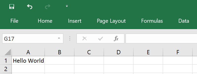
2. As you see, column “A” was resized so “Hello World” fits inside. Easy, isn't it? Well, not as much as we would like it to be. Let's now change the zoom to 50%:

   

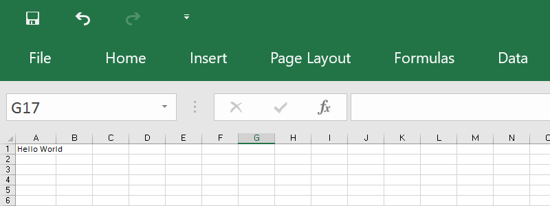
3. Now the text “Hello world” is using part of column “B”. We didn't change anything except the zoom and now text does not fit anymore, in fact, you can autofit it again and column “A” will get bigger.

What happened here? The easy answer is that Excel is resolution dependent. Fonts scale in “steps”, and they look different at different resolutions. What is worse, printing also changes depending on the printer, and as a thumb rule, it is not similar at what you see on the screen.

So, what should a FlexCel autofit do? Make column A the width needed to show “Hello world” at 100% zoom, 96 dpi screen resolution? Resize column A so “Hello world” shows fine when printing? On a dot matrix printer? On a laser printer? Any answer we choose will lead us to a different column width, and there is no “correct” answer.

And it gets better. FlexCel uses GDI+, not GDI for rendering and calculating metrics, and GDI+ is resolution independent. But GDI and GDI+ font metrics are different: for example the space between letters on GDI+ for a font might be less than the space GDI gives to them. You will need less column width to fit “Hello world” on GDI+ than in GDI for that font, so the width calculated by FlexCel(GDI+) will be less than the width calculated by Excel(GDI).

As you can imagine, if we used all this space to describe the problem, is because there is not a real solution. Autofit on FlexCel will try to adapt row heights and column widths so the text prints fine from Excel on a 600 dpi laser printer, but text might not fit exactly on the screen. Autofit methods on FlexCel also provide an “Adjustment” parameter that you can use to make a bigger fit. For example, using 1.1 as adjustment, most text will display inside the cells in Excel at normal screen resolution, but when printing you might find whitespace at the border, since columns or rows are bigger than what they need to be.

Of course, autofit on FlexCel will work fine when printing from FlexCel, since FlexCel is resolution independent and it should always be the same. The problem arises when opening the files in Excel.

And this was the reason we do not automatically autofit rows (as Excel does). Because of the mentioned differences between GDI+ and GDI (and also between GDI at different resolutions), we cannot calculate exactly what Excel would calculate. If we calculated the row height must be “149” and Excel calculated “155”, as all rows are by default autoheight, just opening an Excel file on FlexCel would change all row heights, and probably move page breaks. Due to the error accumulation, maybe in FlexCel you can enter one more row per page, and the header of the new page could land at the bottom of the previous.

The lesson, do the autofit yourself when you need to and on the rows that really need autofit(most don't). If you are using XlsFile, you have XlsFile.Autofit... methods that you can use for that. If you are using FlexCelReport, use the <#Row Height(Autofit)> and <#Column Width(Autofit)> tags to autofit the rows or columns you want.

By default, Excel autofits all rows. So, when opening the file in Excel, it will recalculate row heights and show them fine. But when printing from FlexCel, make sure you autofit the rows you need, since FlexCel will not automatically do that.

Autofitting Merged Cells

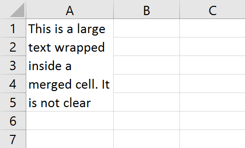
Merged cells can be difficult to autofit, for two basic reasons:

1. If you are autofitting a row, and a merged cell spans over more than one row, which row should be expanded to autofit the cell? Imagine we have the following:

   

   We could make the text fit by enlarging for example row 1, or row 5:

   

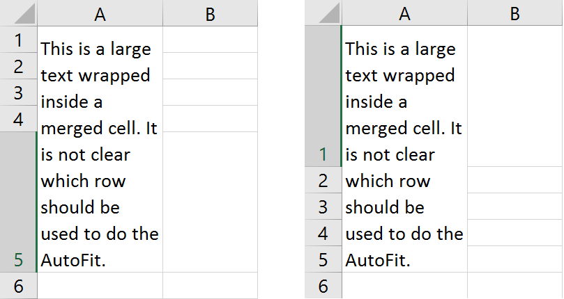
   We could also enlarge all rows by the same amount instead of changing only one row.

   FlexCel by default will use the last row of the merged cell to autofit, since in our experience this is what you will normally need. But you can change this behavior by changing the parameter “autofitMerged” when you call the “Autofit” methods, or, if you are using reports, you can use the <#Autofit settings> tag to do so.

2. The second issue is that probably because of issue 1, Excel will never autofit merged cells. Even in cases where there would be no problem doing so, for example you are autofitting a row and the merged cell has only one row (but 2 columns). In all of those cases, Excel will just make the row the standard height. So, if you apply FlexCel autofitting but leave the autofit on, when you open the file in Excel, Excel will try to re-autofit the merged cell, and you will end up with a single-size row always. So, when autofitting rows with merged cells in FlexCel make sure you set autofitting off for Excel. You don’t need to do this for columns, since they don’t autofit automatically in Excel.

Note

All the above was done in rows for simplicity, but it applies the same to columns and merged cells over more than one column.

Preparing for Printing

After creating a spreadsheet, one thing that can be problematic is to make it look good when printing or exporting to PDF.

Making the sheet fit in one page of width

This is probably the first thing you should do when preparing most documents for printing. Go to the “Page Layout” tab in the ribbon, and look at the “Width” and “Height” boxes

Make the “Height” box “Automatic, to allow your document have as many pages as it needs. You can do this directly in Excel when using Templates to create your documents, or you can do this in FlexCel API by setting TExcelFile.PrintToFit = true, TExcelFile.PrintNumberOfHorizontalPages = 1, and TExcelFile.PrintNumberOfVerticalPages = 0.

Repeating Rows and Columns at the top

Another useful thing you can do is press the “Print Titles” button to access the “Page Setup” dialog. There you can set up some rows and columns to be repeated on every page.

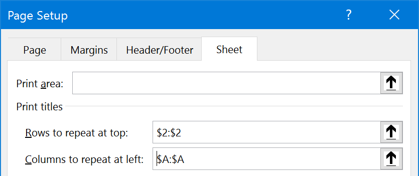
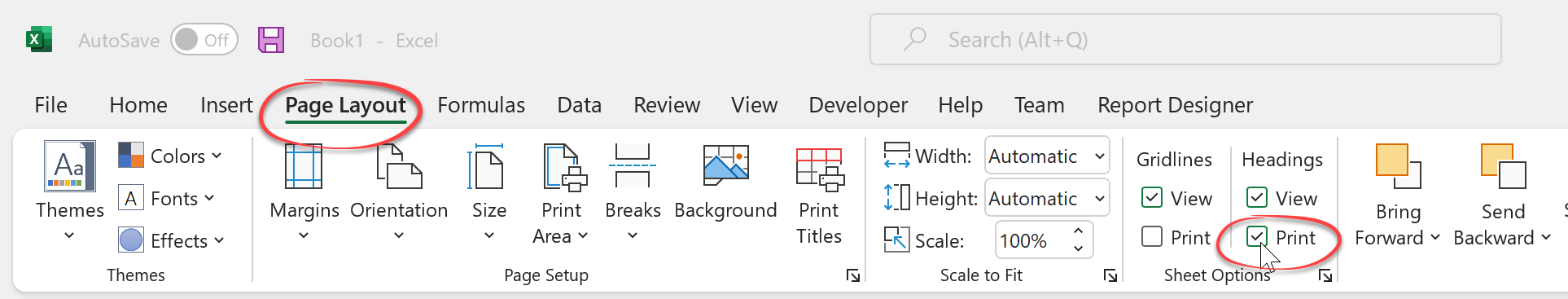
This way your tables can keep their headers in every page. By the way, while you are in the “Sheet” tab, you might want to look at the option to print the gridlines or the column and row headings (The “A”, “B”, etc. at the top and “1”, “2”, etc. numbers at the left of the sheet)

You can do this directly in Excel when using Templates to create your documents, or you can do this in FlexCel API by writing something like this:

  xls.SetNamedRange(TXlsNamedRange.Create(TXlsNamedRange.GetInternalName(TInternalNameRange.Print_Titles), SheetIndex, 0, '=1:2,A:B'));

to set up the rows and columns to repeat, or set TExcelFile.PrintGridLines = true and TExcelFile.PrintHeadings = true to set up printing of gridlines and headings.

Using Page Headers/Footers

Besides repeating rows and columns, you can also add headers and footers from the page setup dialog. One interesting feature in Excel XP or newer is the ability to include images in the page headers or footers. As those images can be transparent, you can have a lot of creative ways to repeat information on every sheet.

From FlexCel API, use the TExcelFile.PageHeader and TExcelFile.PageFooter properties to set the header and footer text. If using a template, you can just set those things in the template.

Cell indentation

The problem

Cell indentation in Excel doesn't work the way most of us would expect it, and in this section we will cover what is wrong and how we tried to fix it.

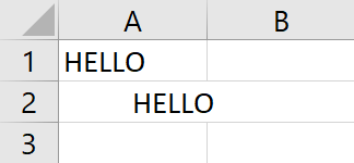
To understand the problem, let's create a new blank document in Excel, and write the word "HELLO" in cells A1 and A2:

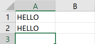
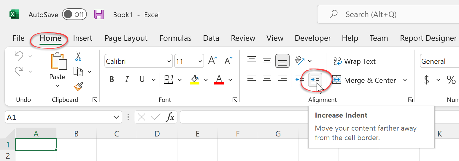
Now, let's give the cell A2 an indentation of 3. You can do this by clicking the indent button in the ribbon 3 times:

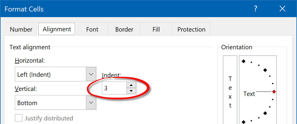
Or by right-clicking the cell, selecting "Format Cells..." and in the "Alignment" tab setting the indent to 3:

No matter how you did it, now the file should look like this:

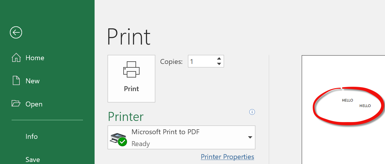
Now let's try to do a print preview. Go to File->Print and it should look like this:

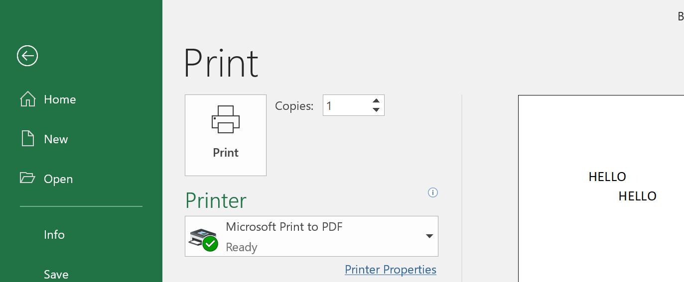
As you can see, the image looks similar (if not exactly the same) to what was shown on the screen, with the "H" in cell A2 roughly below the "O" in cell A1. We are used to small differences between what you see and what is printed, so up to now, everything is fine.

But now, let's change the Print Scale to 50%. Go to the page setup dialog, and change the print scale:

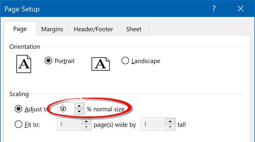
And now we get:

Now, the "H" in cell A2 is way more to the right from the "O" in A1 than before. What happened? We just changed the print scaling, and the layout of the document changed. This is not how we generally expect scaling to work. Going a little more in depth, what happened was that Excel reduced all element sizes, fonts, etc. by 50%, but left the indentation the same. We can see it more clear if we superimpose the 50% and 100% print preview images and zoom in:

The absolute value of the indentation remained the same, and didn't reduce by 50% like everything else. This causes the layout to break.

Note

When "Print Headings" is selected:

Then Excel behaves differently and it scales the indentation proportional to the print scale:

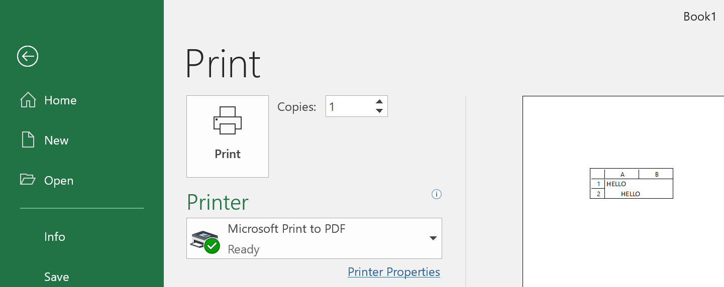
But printing with "print headings" on isn't common, so for most cases, we can say that the indentation doesn't scale with the print scale.

The solution

Up to version 6.23, FlexCel copied the Excel behavior and didn't scale the cell indentation together with the rest of page elements (it wasn't the exact Excel behavior as FlexCel didn't scale either even if print page headings was selected, but printing with page headings is rare).

This original FlexCel behavior matched Excel (and FlexCel has always been about matching Excel even with Excel bugs), but it caused a lot of issues. The most evident one, of course, was that the layout would break when changing the page scaling, and text that was aligned at 100% scaling would become unaligned at 75%.

But there were more subtle issues too: For example FlexCel autofitting runs at 100% scaling (because you can't know at autofitting time which will be the final page scaling). So if you autofitted a column in a page designed to be printed at 75% scaling, it might happen that the exported pdf file couldn't fit the text anymore and had to be printed in 2 lines. Because the autofit was done at 100% and the exporting at 75%, and the indentation is not proportional to the scale like everything else, the free space in the cell is smaller at 75%.

So starting with FlexCel 6.24, we introduced a new Property named TExcelFile.CellIndentationRendering which you can now use to tell FlexCel how to deal with cell indentation and scaling. It offers 3 options:

• The new default behavior: Always scale indentation with page scale.
• The old FlexCel behavior: Never scale indentation with page scale.
• The Excel behavior: Scale indentation only if printing headings, don't scale otherwise.

Important

This is a breaking change in FlexCel 6.24, in that it might break "pixel-perfect" layouts of files with small zoom and cell indentations. It isn't likely to affect you because the new indentations are smaller at smaller zooms, and so more text will fit than before. But if you want to revert to the old behavior, just change TExcelFile.CellIndentationRendering

Conclusion

What we can get from this section is: If you can control the files you are creating, try to avoid using cell indentation in Excel. Cell indentation in Excel is simply broken, and we can fix it on our side, but we can't fix Excel.

Cell indentation also doesn't work all all with Google docs (at the time of this writing), and in Libre/OpenOffice it scales with the print scaling. So using cell indentation will also reduce the portability of your files to other Spreadsheet apps.

If you can't avoid cell indentation, review which value of TExcelFile.CellIndentationRendering is better for you.

Intelligent Page Breaks

Excel offers the ability to include page breaks, but it has no support for any kind of “smart” page breaks that will only break if there is a need for it.

Let's look at an example:

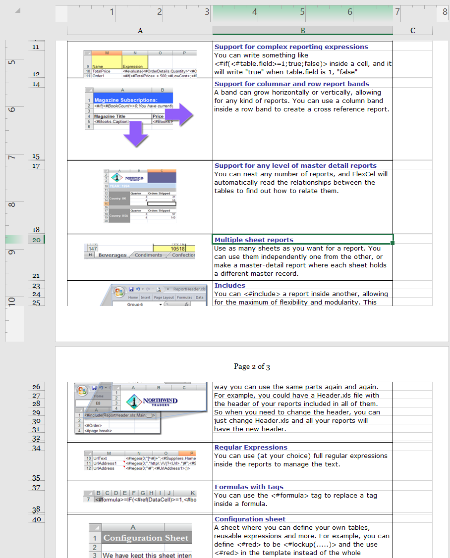
Here, the image in page 1 is being cut in the middle by a page break, so part of it appears on page 1 and part on page 2. While this is no problem when looking at the spreadsheet in Excel, it is clearly not what we want when printing or exporting to PDF. We want to place a page break before that image, so it prints completely in page 2. However, we don't want to put a break before every image, since we can print many in page 2. We need page breaks that only apply when the image does not fit in the current page.

FlexCel offers a way to deal with this. In short, you need to say which rows or columns you would like to keep together by calling TExcelFile.KeepRowsTogether or TExcelFile.KeepColsTogether, and once you have finished creating your file, call TExcelFile.AutoPageBreaks to paginate your whole document and create page breaks in a way your rows and columns are kept together as much as possible.

Note

The call to AutoPageBreaks must be the last before saving your file, so the document is in its final state. If you insert rows or autofit things after calling AutoPageBreaks then the page breaks will be moved out of place. Remember that this is not an Excel feature, so it is simulated by dumb page breaks in Excel, and once set, those page breaks will remain at where they were.

The Widow / Orphan problem

When paginating a document there are actually two similar but different things: widow and orphan lines. In the example above we saw orphan lines, that is, rows that have their “parents” in the previous sheet. But there are also widow lines, and those are rows that are alone in a sheet because the lines below are in a different group, as shown in the following image:

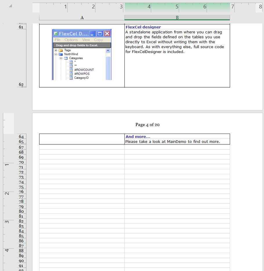
In this example, sheet 4 is almost empty, because there are only two lines from the current group on it, and the next group starts at the next page.

When there is so little written on one page, you will normally want to start the next group on the same page instead of having an empty sheet.

And you can control this in FlexCel with the “PercentOfUsedSheet” parameter when you call AutoPageBreaks. PercentOfUsedSheet defaults at 20, which means that in order to add a page break, the page must be filled in at least 20%.

In the example above, no page break would be made on page 4, since the 20% of the sheet has not been used yet, and so the next group would start on page 4 too. If you set the PercentOfUsedSheet parameter to 0% there will be no widow control, and the next group will start on page 5 no matter if page 4 has one single line.

Setting PercentOfUsedSheet at 100% means no widow or orphan control at all, since in order to set a page break the 100% of the page must have been used, so FlexCel has no margin to add the page breaks. It will not be able to set the page break somewhere before the 100% of the page, so all page breaks will be set at the last row, and it will not be able to keep any rows together. You are advised to keep the PercentOfUsedSheet parameter around 20%

The different printers problem

As explained in the Autofitting Rows and Columns section, Excel prints different things to different printers, and even with the same paper size, some printers have different printing sizes. Printers can have "hard margins" which are places of the sheet where they can't physically print (for example because that part of the sheet is what the printer uses to grab the paper) and this can reduce the effective printing size of the page.

This can be problematic, since a document calculated to have breaks every 30 cm, will have a lot of widow lines if printed in a page with an effective 29.5 cm printing area:

As you can see in the images above, reducing a little the page height might cause the last row not to enter on that page and be printed in the next. As FlexCel added an automatic page break after that row (so it would break correctly with the 30 cm it used for the calculation), you end up with an empty page with only one row.

To solve this issue, the second parameter to AutoPageBreaks is the percentage of the page that will be used by FlexCel to calculate the page breaks. It defaults at 95%, which means that it will consider a page 30 cm tall to be 30*0.95 = 28.5 cm, and calculate the page breaks for that sheet. So it will print correctly in a 29.5 cm sheet.

When calculating the page breaks to directly export to PDF you can keep this parameter at 100%, since FlexCel is resolution independent, and it will not have this issues. But when calculating the page breaks to print from Excel, you need to have a smaller value here so it can fit in all the printers where you might print this sheet. Normally if targeting only laser printers you can have a larger value like 99%, but when other kinds of printers can be used it might be wise to lower this value.

Using different levels of “Keep together”

Normally just marking the rows you want to keep together and then calling AutoPageBreaks should be enough for most cases. But sometimes you might have more than one “keep together” level to keep, and you can set this as one of the parameters in KeepRows/ColsTogether.

Imagine you have a master-detail report with a list of stores, then the customers of each store and the orders for each customer. You might want to keep all customers of a store together on one page, but if that is not possible, at least keep the orders together. You can do this by assigning a level of “2” to the orders, and a level of “1” to the customers. The actual numbers don't matter, you could use a level of “10” for orders and “5” for customers. The only important thing is that one level is bigger than the other.

When you assign different levels to different rows, FlexCel will try to keep lower levels first, but if not possible, it will try to fit at least the higher ones.

Inserting and copying Rows with a “keep together” level

Inserting and copying rows works as expected, when you copy a group of rows with a level of 2 and insert them in another place, the “2” level will be copied. It also works when copying across different files, but you need to copy full rows in any case. When copying ranges that are not the complete rows, those values will not be copied, as expected.

Debugging Intelligent Page Breaks

Intelligent page breaks are a tested technology: They work well and we aren't aware of bugs on its implementation. But sometimes, they might produce results that look wrong at first sight. And when they aren't working as you expect them to, it helps to understand a little more in depth what is going on under the hood.

Note

For simplicity in this section we are going to speak always about row breaks, but the column breaks work in a similar fashion.

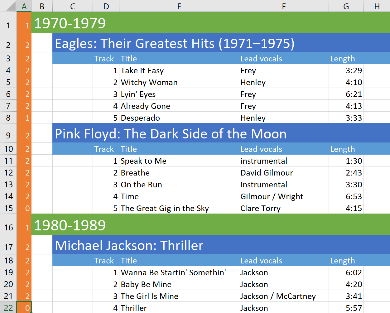
The first thing to notice is that intelligent page breaks work by marking the rows (or columns) to be kept together with a level. So let's imagine we have this file: A master-detail report with the best selling albums in each decade and some of their songs:

We want to keep together every decade on its own page, or if not possible, at least keep together every full album. For this we can define the following keep together ranges:

1. Rows 1 to 15, level 1
2. Rows 16 to 22, level 1
3. Rows 2 to 8, level 2
4. Rows 9 to 15, level 2
5. Rows 17 to 22, level 2

Or with code:

  xls.KeepRowsTogether(1, 15, 1, false);
  xls.KeepRowsTogether(16, 22, 1, false);
  xls.KeepRowsTogether(2, 8, 2, false);
  xls.KeepRowsTogether(9, 15, 2, false);
  xls.KeepRowsTogether(17, 22, 2, false);

Tip

Of course the code above is not how you will set the intelligent page breaks in normal use. In real code you will be using some kind of loop, or inserting and copying rows, or setting keep together ranges in reports. But the effect once that is done is similar to manually calling TExcelFile.KeepRowsTogether with the values above.

To better understand what is happening, let's see now how FlexCel translates those TExcelFile.KeepRowsTogether commands into its data model. Conceptually it is simple: When you call TExcelFile.KeepRowsTogether for rows 1 to 15 to be level 1 (as in the first line of the example above), FlexCel will mark rows 1 to 14 to be level 1. There was no typo in the previous line: Marking rows 1 to 15 to be level 1 makes FlexCel mark rows 1 to 14 to be level 1. If we add a small column to visualize the marked rows after marking rows 1 to 15, the file should look like this:

So why is FlexCel marking one less row than what you marked? This should become clear when we call the second KeepTogether line to keep rows 16 to 22. After that call, the file will look like this:

Note how there is a 0 at row 15. If the first call to KeepRowsTogether had marked rows 1 to 15 instead of 14, then row 15 would also have a 1 there. And the full rows 1 to 22 would be marked as level 1, the same as if we had just caller KeepRowsTogether from row 1 to 22. But we didn't make a single call from rows 1 to 22. We marked rows 1 to 15 and 16 to 22. We want FlexCel to know that it can break the page at row 15 if it needs to. When running the actual page break algorithm, FlexCel will take into account that missing row, and still know that row 15 belongs together with row 14 even if internally row 15 is marked with level 0.

Marking one less row than the rows you mark allows you to mark 2 consecutive ranges like 1:5 and 5:10 and have them still be separated ranges instead of becoming a single 1:10 range

Important

You might be wondering why we spent so much time explaining an implementation detail like how FlexCel maps your calls to KeepRowsTogether to its internal data model. After all, it shouldn't really matter how FlexCel internally models your commands. And in most cases, it won't actually matter.

But this section is about debugging page breaks, and you will need to debug them when something went wrong. There are 2 reasons why it helps to understand the internal representation FlexCel does from your commands:

1. The fact that when you mark rows 1 to 2 only row 1 is marked is the most common cause of discrepancies between what you think FlexCel should do and what FlexCel actually does. In most cases, it will work just as you expect it to work and you don't need to think in the internals. Just mark the block you want to keep together and know they will be kept together. But if it is not working as it should, then it likely is caused by this.

2. As we will see shortly, when debugging reports you will be able to see this internal FlexCel representation, so you will need to understand how it is implemented.

Ok, now let's run the full code and add the lines that call KeepRowsTogether with level 2. This is how the file will end up marked:

When FlexCel runs the intelligent page breaks in this page it will:

1. Try to fit all level 1+ rows on one page, adding an extra row because the rows marked are one less. So, the first block of levels >=1 go from 1 to 14. Adding the extra row, FlexCel will try to fit the block 1 to 15 in a single page.
2. If it can't fit rows 1 to 15 in a single page, it will try with level 2+. The first block of level 2+ goes from rows 2 to 7. So it will try to fit the rows 1 to 8 in a single page. And so on.

After diving in the technical details, we can see it is doing what we told it to do. It first tries to fit rows 1 to 15 (the first KeepRowsTogether call), then 2 to 8 (the third KeepRowsTogether call) and then the others.

Now, wouldn't it be nice to be able to directly see FlexCel's internal representation for those cases where the page breaks aren't working as they should? Without having to do it manually as we did here?

The good news is that yes, it is possible. FlexCel has commands for both the API and reports that let you see the levels that FlexCel sees. To understand those levels, you just need to remember that the last line of each keep together block isn't marked, but considered anyway to belong to the group.

When using the API, FlexCel has 2 commands: TExcelFile.DumpKeepRowsTogetherLevels and TExcelFile.DumpKeepColsTogetherLevels. The first one will write all row levels in the column you specify, and the second will do the same for columns. Looking at the actual numbers should help understanding how FlexCel sees your blocks.

When using reports you have two ways to enter intelligent page breaks debug mode, similar to Report Debug mode and Errors in result file modes:

1. You can set TFlexCelReport.DebugIntelligentPageBreaks to true in the code.
2. You can write a tag <#Debug Intelligent Page Breaks> anywhere in the Expressions column of the config sheet.

As with the debug mode and Errors in Result File mode, the second way to enter Debug Intelligent Page Breaks mode is better when you are editing a template and want to do a debug without modifying the code, while the first way is better if you are automating testing and do not want to modify the templates.

Note

When inserting and deleting rows, FlexCel doesn't just insert or delete them, but adapts the levels so they still behave as you would expect. This can cause issues understanding why a row ended up with a level. For example, if in our last screenshot we removed row 8, a naive implementation would just remove that row, and the group that ends at row 8 (Eagles) would be joined with the group that starts at row 9 (Pink Floyd). But when you remove that row, FlexCel is smart enough to make row 7 level 1, so the file still behaves as it should and you still have one group for the Eagles and one for Pink Floyd. The fact that you removed a song from the Eagles group is no reason for it to become one big group with Pink Floyd.

While FlexCel always tries to do "the right thing", sometimes the right thing might not be what you expected, or it might not be the right thing for a specific situation. This is why being able to see the actual values of levels added by FlexCel can be so helpful.

Using Excel's User-defined Functions (UDF)

Introduction

User-defined functions in Excel are macros that return a value, and can be used along with internal functions in cell formulas. Those macros must be defined inside VBA Modules, and can be in the same file or in an external file or addin.

While we are not going to describe UDFs in detail here, we will cover the basic information you need to handle them with FlexCel. If you need a more in-depth documentation in UDFs in Excel, there is a lot of information on them everywhere.

So let's start by defining a simple UDF that will return true if a number is bigger than 100, false otherwise.

We need to open the VBA editor from Excel (Alt-F11), create a new module, and define a macro inside that module:

Function NumIsBiggerThan100(Num As Single) As Boolean
    NumIsBiggerThan100 = Num > 100
End Function

And then write “=NumIsBiggerThan100(120)” inside a cell. If everything went according to the plan, the cell should read “True”

Now, when recalculating this sheet FlexCel is not going to understand the “NumIsBiggerThan100” function, and so it will write #Name? in the cell instead. Also, if you want to enter “=NumIsBiggerThan100(5)” say in cell A2, FlexCel will complain that this is not a valid function name and raise an Exception.

In order to have full access to UDFs in FlexCel, you need to define them as a class in Delphi or C++ Builder and then add them to the recalculation engine.

Step 1: Defining the Function in Delphi

To create a function, you need to derive a class from TUserDefinedFunction, and override the Evaluate method. For the example above, we would create:

type
  TNumIsBiggerThan100 = class (TUserDefinedFunction)
  public
    constructor Create;
    function Evaluate(const arguments: TUdfEventArgs;
                      const parameters: TFormulaValueArray): TFormulaValue; override;
  end;

{ TNumIsBiggerThan100 }
constructor TNumIsBiggerThan100.Create;
begin
  inherited Create('NumIsBiggerThan100');
end;

function TNumIsBiggerThan100.Evaluate(const arguments: TUdfEventArgs;
                             const parameters: TFormulaValueArray): TFormulaValue;
var
  Err: TFlxFormulaErrorValue;
  Number: RealNumber;
begin
  //Do not define any global variable here.

  //Check we have only one parameter
  if not CheckParameters(parameters, 1, Err) then
    exit(Err);

  //The parameter should be a double.
  if not TryGetDouble(arguments.Xls, parameters[0], Number, Err) then
    exit(Err);

  Result := Number > 100;
end;

As you can see, it is relatively simple. Some things worth noting:

1. Don't use global variables inside Evaluate: Remember, the Evaluate() method might be called more than once if the function is written in more than one cell, and you cannot know the order in which they will be called. Also if this function is registered to be used globally, more than a thread at the same time might be calling the same Evaluate method for different sheets. The function must be stateless, and must always return the same value for the same arguments.

2. As you can see in the help for the TUserDefinedFunction.Evaluate method, the evaluate method has two arguments. The first one provides you with utility objects you might need in your function (like the TXlsFile where the formula is), and the second one is a list of parameters, as an array of TFormulaValue.

   Each object in the parameters array might be a null, a Boolean, a String, a Double, a TXls3DRange, a TFlxFormulaErrorValue, or a 2 dimensional array of objects, where each object is itself of one of the types mentioned above.

   While you could manually check for each one of the possible types by manually checking all possible types for each parameter, this gets tiring fast. So the TUserDefinedFunction class provides helper methods in the form of “TryGetXXX” like the TUserDefinedFunction.TryGetDouble method used in the example.

3. There is the convention in Excel that when you receive a parameter that is an error, you should return that parameter to the calling function. Again, this can be tiring to do each time, so the TUserDefinedFunction class provides a TUserDefinedFunction.CheckParameters method that will do it for you.

   The only time you will not call TUserDefinedFunction.CheckParameters as the first line of your UDF is when you are creating a function that deals with errors, like “IsError(param)”, that will return true when the parameter is an error.

4. Do not throw Exceptions. Exceptions you throw in your function might not be trapped by FlexCel, and will end in the recalculation aborting. Catch all expected exceptions inside your method, and return the corresponding TFlxFormulaErrorValue when there is an error.

Step 2: Registering the UDF in FlexCel

Once you have defined the UDF, you need to tell FlexCel to use it. You do this by calling TExcelFile.AddUserDefinedFunction in a TExcelFile object. Once again, some points worth noting:

1. You need to define the scope of your function. If you want it to be globally accessible to all the TExcelFile instances in your application, call TExcelFile.AddUserDefinedFunction with a “Global” TUserDefinedFunctionScope. If you want the function to be available only to the TExcelFile instance you are adding it to, specify “Local”. Global scope is easier if you have the same functions for all the files, but can cause problems if you have different functions in different files. Local scope is safer, but you need to add the functions each time you create a TExcelFile object that needs them. If you are unsure, probably local scope is better.

2. You also need to tell FlexCel if the function will be defined inside the same file or if it will be in an external file. This is not really needed for recalculating, but FlexCel needs to know it to enter formulas with custom functions into cells.

There are four things you can do with formulas that contain UDFs, and there are different things you need to do for each one of them:

1. Retrieve the formula in the cell: You do not need to do anything for this. FlexCel will always return the correct formula text even if you do not define any udf. If the file was calculated when saved in Excel (the default), then FlexCel will also return the correct value of the formula.

2. Copy a cell from one place to another. Again, there is no need to do anything or define any UDF object. FlexCel will always copy the right formula, even if copying to another file.

3. Calculate a formula containing UDFs. For this one you need to define a UDF class describing the function and register it. You do not need to specify if the formula is contained in the sheet or stored in an external addin.

4. Enter a formula containing a UDF into a sheet. In order to do this, you need to define and register the UDF, and you must specify if the function is stored internally or externally.

For more examples on how to define your own UDFs, please take a look at the Excel User Defined Functions API demo.

Note

Even when they look similar, UDFs are a completely different thing from Excel Built-in functions. Everything said in this section applies only to UDFs, you cannot use this functionality to redefine a standard Excel function like “Sum”. If recalculating some built-in function is not supported by FlexCel just let us know and we will try to add the support, but you cannot define them with this.

Returning Arrays from UDFs

If you are using array formulas, you might need to return an array from your user-defined function. It is no really different from the standard UDFs, but you need to return a 2-dimensional array of objects from the Evaluate method.

So if we wanted to define a simple UDF that returns an array with 4 fixed numbers, we could define a function like the following:

type

  THelloFlexCelImpl = class (TUserDefinedFunction)
  public
    constructor Create;
    function Evaluate(const arguments: TUdfEventArgs; const parameters: TFormulaValueArray): TFormulaValue; override;
  end;

{ THelloFlexCelImpl }
constructor THelloFlexCelImpl.Create;
begin
  inherited Create('hello_flexcel');
end;

function THelloFlexCelImpl.Evaluate(const arguments: TUdfEventArgs; const parameters: TFormulaValueArray): TFormulaValue;
var
  Err: TFlxFormulaErrorValue;
begin  
   //Do not define any global variable here.

   //Check we have no parameters
  if not CheckParameters(parameters, 0, Err) then
    exit(Err);
  
   // Note that we return a 2-dimensional array of objects,
   // even if the array is 1-dimensional.
  exit(TFormulaValueArray2.Create(TSingleFormulaValueArray.Create(8, 9, 10, 11)));
end;

And then, in FlexCel we could use the following code to enter formulas that use the UDF:

  xls.AddUserDefinedFunction(TUserDefinedFunctionScope.Global, TUserDefinedFunctionLocation.External, THelloFlexCelImpl.Create);
  xls.SetCellValue(2, 1, TFormula.Create('{=HELLO_FLEXCEL()}', TFormulaValue.Empty, TFormulaSpan.Create(1, 4, true)));

Recalculating Linked Files

FlexCel offers full support for recalculating linked files, but you need to add some extra code to make it work. Everything we will discuss here is about TExcelFile objects, but you can also use this on reports. Just run the reports with TFlexCelReport.Run(xls).

The main issue with linked files is telling FlexCel where to find them.

Normally, if your files are on a disk, there should be not much problem to find a linked file. After all, that information is inside the formula itself, for example if FlexCel finds the formula:

='..\Data\[linked.xls]Sheet1'!$A$3 * 2

inside a cell, it could automatically find “..\Data\linked.xls”, open it, and continue with the recalculation.

In fact, there are two problems with that approach:

1. Files might not be in a filesystem. FlexCel allows you to transparently work with streams instead of physical files, and so you might have for example the files stored in a database. In this case, trying to find “..\Data\linked.xls” makes no sense, and FlexCel would fail to recalculate.

2. Much more important than problem 1, this approach could imply an important security risk.

   Blindly following links in an unknown xls file is not a smart idea. Let's imagine that you have a web service where your user submits an xls file, you use FlexCel to convert it to PDF, and send back the converted PDF to him. If that user knows the location of an xls file in your server, he could just submit a hand-crafted xls file filled with formulas like:

      ='c:\Confidential\[BusinessPlan.xls\]Sheet1'!A1,
      ='c:\Confidential\[BusinessPlan.xls\]Sheet1'!A2,
      ...
   

   On return you would supply him with a PDF with the full contents of your business plan. What is even worse, since FlexCel can read plain text files, he might also be able to access any text file in your server. (Imagine you are running on Linux and formulas pointing to /etc/passwd)

Note

You might argue that in a well-secured server your application should not have rights on those files anyway, but on security, the more barriers and checks you add the better. So you should have a way to verify the links inside an arbitrary file instead of having FlexCel opening them automagically.

Because of reasons 1) and 2), FlexCel by default will not recalculate any linked formula, and just return “#NA!” for them. Note that in most cases you will want to leave this that way, since most spreadsheets don't have linked formulas anyway, and there is no need to add extra security risks just because.

But if you do need to support linked files, adding that support is easy.

The first thing you need to do is to create a TWorkspace object. Workspaces are collections of XlsFile objects, and when you recalculate any of the files in a Workspace, all the others will be used in the recalculation (and be recalculated) too.

So the simplest and more secure way to recalculate linked files is to create a Workspace, add the needed XlsFile objects inside, and just recalculate any of the files as usual. For example:

var
  work: TWorkspace;
begin
  //The Workspace will own the TXlsFile objects,
  //so we won't need to free them.
  //If we set the parameter to false,
  //we would have to manually free the TXlsFile objects.
  work := TWorkspace.Create(true);
  try
    work.Add('xls1', TXlsFile.Create('File1.xlsx'));
    work.Add('xls2', TXlsFile.Create('File2.xlsx'));
    work.Add('xls3', TXlsFile.Create('File3.xlsx'));

   //Either work.Recalc, xls1.Recalc, xls2.Recalc or xls3.Recalc will recalculate all the files in the workspace.
    work.Recalc(true);
  finally
    work.Free;
  end;
end;

In the example above, we opened two files and added them to a workspace, giving each one a name to be used in the recalculation process. Note that here we don't have issues 1) or 2) at all. We could have opened those files from a stream and it would be the same, since the name “file1.xls” needed to calculate is actually given in the “work.Add()” method. The actual name and location (if any) of the file “file1.xls” is irrelevant. And also we don't have the security concern of FlexCel opening files by itself, since we opened the files we wanted, and FlexCel will not open any more files.

Now, in some cases you don't know a priori which files you are going to need in order to recalculate the file, and so you cannot use the approach above. In those cases, you still use the Workspace object, but you assign an event where you load those files when FlexCel asks for them. The code would be something like:

var
  Work: TWorkspace;
...
   //Create a workspace
  Work := TWorkspace.Create;
  try
    //Add the original file to it
    Work.Add(TPath.GetFileName(FileName), TXlsFile.Create(FileName));
    
  //Set up an event to load the linked files.
    Work.LoadLinkedFile := LoadLinkedFile;
    
   //Recalc will recalculate xls1 and all the other files used in the recalculation. 
   //At the end of the recalculation, all the linked files will be loaded in the workspace, 
   //and you can use the methods in it to access them. 
    Work.Recalc(true);
  finally
    Work.Free;
  end;

In the LoadLinkedFile event you can load the needed files, checking that they are not trying to access folders they shouldn't be looking to. For example, remove all path information and only load files from the same folder the original file is. Or only allow paths that are children of the path of the main file, or maybe paths from an allowed list of paths. The choice is yours.

The LoadLinkedFile event would be declared like this:

procedure LoadLinkedFile(const sender: TObject; const e: TLoadLinkedFileEventArgs);
begin
   //Load the file here checking it is a allowed file.
   //In this example we will just load the linked file
   //Without checking it, but this is only to keep the example simple.
  e.Xls := TXlsFile.Create(e.FileName);
end;

You can take a look at the Validate Recalc demo to see a real implementation of this. In that example there is no validation of the loaded filenames, but just because it is an application designed to run locally with full trust.

Important

If XlsFile objects can consume lots of memory, Workspace objects can consume much more, since they are a collection of XlsFiles themselves. So same as with XlsFile objects, don't leave global Workspace objects hanging around. Free them as soon as possible.

Take also a look at the example Recalculation of linked files for more information.

Miscellanea

Using FlexCel inside a dll

Sometimes you might want to use FlexCel inside a dll, and call it from other Windows application.

For those cases, you must be aware that FlexCel in Windows uses GDI+, and GDI+ must be initialized from your main application before you call the methods in the dll. (For more information, please look at the remarks at http://msdn.microsoft.com/en-us/library/windows/desktop/ms534077(v=vs.85).aspx )

FlexCel provides two methods that will do this initialization for you: FlexCelDllInit and FlexCelDllShutdown. At the time of this writing all those methods do is to initialize and shutdown GDI+ when in Windows, and they do nothing in other platforms. But in the future they might be expanded to do more stuff, so it is a good practice to call them whenever you are going to call a dll which uses FlexCel, if you aren’t using FlexCel in your main application.

If you are encapsulating FlexCel methods inside a dll, make sure to expose FlexCelDllInit and FlexCelDllShutdown in the dll, and call those methods when initializing and shutting down your application.

Avoiding the “Want to save your changes?” dialog on close.

By default, FlexCel will not identify the xls/x files it generates as having been recalculated by any Excel version. This will cause Excel to recalculate the file on open, and when closing the file, it will show the following dialog:

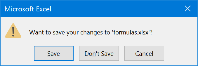
This will always happen when you save a file with formulas. We choose this as the default mode because we can’t know which formulas your file has, and while we support over 300 Excel functions, you might be using something we don’t support, or some VBA macro function that you didn’t re-implement in FlexCel, or some linked files without setting up FlexCel to recalculate linked files. So the safest default is to leave Excel to recalculate files on open, and this has the side effect of this dialog popping up when you try to close the file.

If you know the formulas you are using are all supported, and you would like to get rid of this dialog, you can tell FlexCel to identify the file as having been saved by a specific Excel version.

So you can for example do:

TExcelFile.RecalcVersion = TRecalcVersion.Excel2019;

or if using reports:

TFlexCelReport.RecalcVersion = TRecalcVersion.Excel2019;

Once you do this, any Excel version equal to or older than Excel 2019 will not recalculate the file on open, trusting the recalculation FlexCel did, and it won’t show the dialog on close.

Newer Excel versions will still recalculate and ask for save on close.

Note

If you want to use the always use the latest version supported by FlexCel, you can specify TRecalcVersion.LatestKnownExcelVersion. This value is set to the latest Excel version FlexCel knows about, so when you update FlexCel it will update automatically without you having to modify your code.

The other special value is TRecalcVersion.SameAsInputFile. This value means to use the value in the file you are using as a template. Let's imagine that you have an old FlexCel version which supports up to Excel 2013, and you had a file saved in Excel 2016. With this value, FlexCel will identify the file as saved as Excel 2016, even if it doesn't know about it. It will just copy the value from the input file which was in Excel 2016.

Closing Words

We hope that after reading this document you got a better idea on the basic concepts of using the FlexCel API. Concepts mentioned here (like XF format indexes) are basic to use FlexCel, so it is important that you get them right.

And one last thing. Remember that FlexCel API's main strength is that it modifies existing files; it doesn't use the traditional approach of one API for reading the file and another for writing. In fact, FlexCel doesn't even know how to create an empty file. When you call TExcelFile.NewFile, you are really reading an empty xls file embedded as a resource. You are always modifying things.

Take advantage of this. For example, let's say you want to save a macro on your final file. There is no support on FlexCel for writing macros. But you can create the macro on Excel and save it to a template file, and then open the template with FlexCel instead of creating a new file with NewFile.

Use Excel and not FlexCel to create the basic skeleton for your file. Once you have all of this on place, modify it with FlexCel to add and delete the things you need. This is what FlexCel does best. And of course, remember that you can use TFlexCelReport for creating files, designing your files in Excel in a visual way.